Microsoft excel tutorial for beginner to advanced learners

Microsoft Excel is a software application that provides an electronic sheet.

Where you can create Result Sheet, Pay Sheet, Electricity Bill Sheet, Shop Bill Sheet, Attendance Sheet and other accounts sheets.

How to Open Excel?

Click on the Start, and type excel, if MSOffice will already be installed then click on the excel otherwise install it.

or Press the (windows button + R) and press Enter key. A run dialogue box will appear type excel and press the Enter key.

Microsoft Excel Sheet

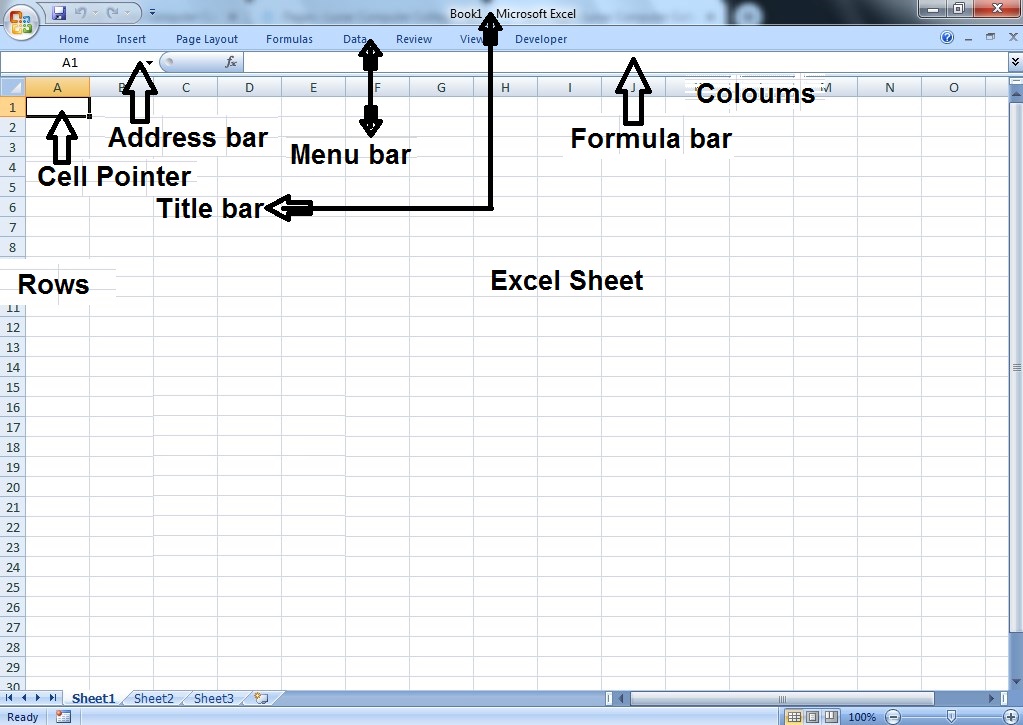
Principles of writing data in Microsoft Excel

In Excel, we add data with the following principles.

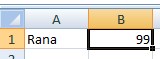
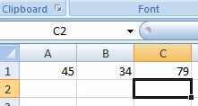
Numeric data, is on the right side of the cell pointer of the Excel sheet, while non-numeric data, is on the left side as shown in the picture above.

How to Add the Numeric Values in the Excel?

There are several ways we can use to add numeric values in Ms Excel.

Using this method you can add two or multi numeric values to Microsoft Excel’s sheet.

Start the formula from = sign in excel

=Cell Address + Cell Address [To add the values in A1 and B1 cells]
=A1+B1

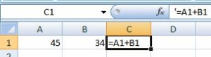
as you will press the Enter key computer will show the result in the C1 cell as shown in the image below.

Add numeric values in a range in Ms Excel

=sum(Start Cell Address:End Cell Address)

To add the values from A1 to G1 in the range]

=sum(A1:G1)

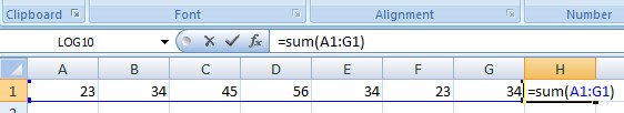
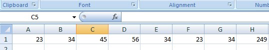
Press the Enter key to see the result in the formula cell

See the image below:

How to Subtract the Numeric Values in the Excel?

=Cell Address-Cell Address
=A1-B1

=sum(Cell Address-Cell Address)
=sum(A1-B1)

How to Multiply the Numeric Values in the Excel?

=Cell Address*Cell Address
=A1*B1

=sum(Cell Address*Cell Address)
=sum(A1*B1)

How to Divide the Numeric Values in the Excel?

=Cell Address/Cell Address
=A1/B1

=sum(Cell Address/Cell Address)
=sum(A1/B1)

How to find the maximum value from the values in a range?

=max (range)

To find the maximum value from the range A1 to A6 type =max(A1:A6) as shown in the image below.

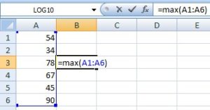
After pressing Enter Computer will type 90 in the formula Cell

How to find the minimum value from the values in a range?

=min (range)

To find the minimum value from the range A1 to A6 type =min(A1:A6) as shown in the image below.

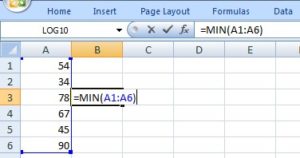
After pressing Enter Computer will type 34 in the formula Cell

How to convert numbers into words in Excel?

In Excel, there are several ways that you can use to change the numbers into the word. But I am explaining the very simple way.

Check the following function 1st.

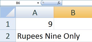
=SpellNumber(9)

or type 9 in cell A1 and put cell pointer on A2 and type =SpellNumber(A1)

if the computer converts 9 into words (Your currency name and Nine) then the function is working as shown in the image below.

If it is not working then follow all the following procedures step by step as shown below.

Download This file

After downloading the file Unzip the File, Right Click on the file and then Click on Extract Here.
Open the extracted folder and copy the file named SpellNumber
Mark the tick sign on the Show hidden file, folders and drives under the Folder Options.
Open the Users folder.
Now open the folder with the name you created.
You will see AppData Folder Open it
Then Open the Roaming folder under the AppData folder.
Under the Roaming folder open the Microsoft Folder.
Finally, open the AddIns folder and Paste that file (SpellNumber) here that you have copied in step 2.
Now open the Microsoft Excel Software application.
Open Excel Options by clicking the upper top left corner MSOffice icon.
Click on Add-Ins
Now click on SpellNumber from the next window.
Click on Go that you will see after, Manage and Excel Add-Ins.
Checked the SpellNumber and Click Ok
Now your =SpellNumber() function is activated.

=SpellNumber (A1)

=SpellNumber (10)

How to Create a Result Sheet in Excel?

Step1. Type Result Sheet in the A1 Cell Address

Step2. Type Result Sheet Sub Headings from S/No to Remarks Starting from A2 to N2, as shown in the image below.

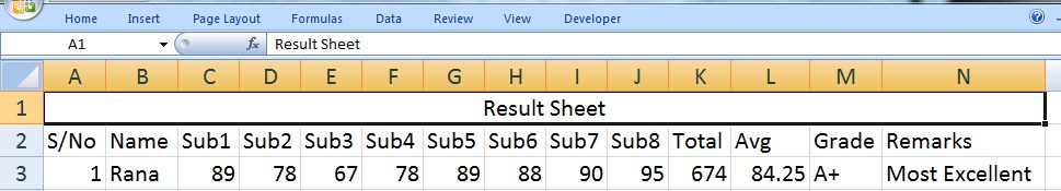
Now type the data as you can see on the above image in row 3. From A3 to J3 Total Avg Grade.

Total, Avg, Grade and Remarks we will get with the help of formulas.

The formula for Total in Excel

Put the cell pointer under the subheading Total on K3 according to the above sample Result Sheet image and type the following formula

=sum(c3:j3) and then press the Enter to get the result.

The formula for Average in Excel

Put the cell pointer under the subheading Avg and type the following formula to get the average of the students’ results while all subjects’ total marks are equal to 100.

=average(c3:j3) and then press the Enter to get the result.

The formula for Grade in Excel

Put cell pointer under the subheading Grade and type the following formula of the grade while (L3) is the cell address of average which you have solved above.

=IF(L3>=80,”A+”,IF(L3>=70,”A”,IF(L3>=60,”B”,IF(L3>=50,”C”,IF(L3>=40,”D”,IF(L3>=33,”E”,”Fail”))))))

The formula for Remarks in Excel

Put cell pointer under subheading Remarks and type the following formula for remarks while (M3) is the cell address of the grade which you have solved above.

=IF(M3=”A+”,”Most Excellent”,IF(M3=”A”,”Excellent”,IF(M3=”B”,”Very Good”,IF(M3=”C”,”Good”,IF(M3=”D”,”Fair”,IF(M3=”E”,”Poor”,”Very Bad”))))))

How to Make a Result Sheet in Excel | English Subtitles |

Video Tutorial

How To Make an Attendance Sheet In Excel?

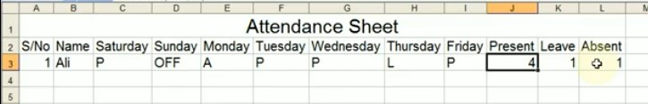
Type Attendance Sheet in A1

Now type S/No in A2, Name in B2, Saturday in C2, Sunday in D2, Monday in E2, Tuesday in F2, Wednesday in G2, Thursday in H2, Friday in I2, Present in J2, Leave in K2 and Absent in L2

And now type 1 in A3, Ali in B3, P in C3, OFF in D3, A in E3, P in F3, P in G3, L in H3, P in I3

Now put the cell pointer in j4 and type =countif(c3:i3,”p”) press Enter, in K4 and type =countif(c3:i3,”L”) press Enter, and in the L4 and type =countif( c3:i3,”A”) press Enter

Video lecture excel attendance sheet

How to use iferror function in excel?

In Microsoft Excel when you divide the value with 0 (zero) or with a string then the computer displays an error (#DIV/0!) as shown in the image below.

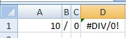
In the upper image as you divided the 10 with 0 using this formula =A1/C1 then the computer provided me with the result #DIV/0!.

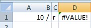
Similarly, if you divide the values with any string in Excel like (10/r) the result will be #VALUE! as shown in the image below.

Now by using the iferror function you can change the error message.

The syntax of iferror function is;

=iferror(A1/C1,0)

You can watch this video to understand the function of iferror.

What is the use iferror function in ms excel?

Prime Number Coding Ms Excel

Type your number in A1 and copy and paste the following code in A2

=IF(AND(A1>1, MOD(A1,2)<>0, MIN(IF(MOD(A1,ROW(INDIRECT(“2:”&INT(SQRT(A1)))))=0,0,1))=1), “Prime”, “Not Prime”)

How to add a real time clock in Excel

Open Excel and press Alt + F11 to open the VBA editor.
In the editor, click Insert and then select Module.
In the module, paste this code:

Dim NextTick As Date

Sub StartClock()
NextTick = Now + TimeValue(“00:00:01”)
Range(“A1”).Value = Format(Time, “hh:mm:ss AM/PM”)
Application.OnTime NextTick, “StartClock”
End Sub

Sub StopClock()
On Error Resume Next
Application.OnTime NextTick, “StartClock”, , False
End Sub

Close the VBA editor by pressing Alt + Q.
Back in Excel, press Alt + F8, select StartClock, and click Run. This will start displaying the real-time clock in cell A1.

If you ever want to stop the clock, just run StopClock in the same way.

SiteMap